Bubonic Plague: Mathematical Modeling Foundations

library(yersinia)
library(ggplot2)
library(dplyr)
library(tidyr)

Introduction

Historical Context

Bubonic plague, caused by the bacterium Yersinia pestis, has been one of history’s most devastating diseases. The “Black Death” of the 14th century killed an estimated 30-60% of Europe’s population, fundamentally altering the course of human history. The disease persists today, with modern outbreaks providing crucial data for understanding its transmission dynamics.

The Role of Mathematical Modeling

Mathematical models help us understand disease transmission mechanisms and predict outbreak patterns. For plague, these models are particularly interesting because they must capture the complex interactions between three populations:

Rats (the primary host)
Fleas (the vector)
Humans (the incidental host)

This vignette explores classical deterministic models based on the foundational work of Keeling & Gilligan (2000), focusing on the rat-flea transmission cycle that drives plague dynamics.

Educational Purpose

Note: This vignette presents reference implementations for educational purposes. These deterministic models provide mathematical foundations for understanding plague transmission. For operational research and realistic population dynamics, the main yersinia package implements advanced stochastic models via run_plague_model().

Mathematical Framework

Basic Components

The model tracks five main variables representing the key populations in plague transmission:

$S_r$ : Susceptible rats
$I_r$ : Infected rats
$R_r$ : Resistant rats
$N$ : Average number of fleas per rat (flea index)
$F$ : Free infectious fleas

Core Equations

The system is described by the following differential equations:

$\begin{align} \frac{dS_r}{dt} &= \underbrace{r_r S_r \left( 1 - \frac{T_r}{K_r} \right)}_{\text{births}} + \underbrace{r_r R_r(1 - p)}_{\text{non-immune births}} - \underbrace{d_r S_r}_{\text{deaths}} - \underbrace{\beta_r \frac{S_r}{T_r}F\left[1-\exp(-aT_r)\right]}_{\text{infections}}\\ \frac{dI_r}{dt} &= \underbrace{\beta_r \frac{S_r}{T_r}F\left[1-\exp(-aT_r)\right]}_{\text{infections}} - \underbrace{(d_r + m_r)I_r}_{\text{death/recovery}}\\ \frac{dR_r}{dt} &= \underbrace{r_r R_r \left(p - \frac{T_r}{K_r}\right)}_{\text{immune births}} + \underbrace{m_r g_r I_r}_{\text{recovery}} - \underbrace{d_r R_r}_{\text{natural death}}\\ \frac{dN}{dt} &= \underbrace{r_f N \left(1 - \frac{N}{K_f}\right)}_{\text{flea reproduction}} + \underbrace{\frac{F}{T_r} \left(1 - \exp(-a T_r)\right)}_{\text{free fleas finding rats}}\\ \frac{dF}{dt} &= \underbrace{(d_r + m_r (1 - g_r)) I_r N}_{\text{free infected fleas from dead rats}} - \underbrace{d_f F}_{\text{infected flea deaths}} \end{align}$

where $T_r = S_r + I_r + R_r$ is the total rat population.

Biological Interpretation

Each term represents a specific biological process:

Rat population dynamics follow logistic growth with carrying capacity $K_r$
Disease transmission occurs through infected flea bites on susceptible rats
Flea dynamics include reproduction on hosts and host-seeking behavior
Resistance inheritance allows some rats to be born with immunity (probability $p$ )
Recovery from infection confers permanent immunity with probability $g_r$

Model Parameters

The parameters capture key biological and epidemiological processes:

Rat Population Parameters

$K_r$ : Rat carrying capacity
$r_r$ : Rat population growth rate (per year)
$d_r$ : Natural death rate of rats (per year)
$p$ : Probability of inherited resistance

Disease Parameters

$\beta_r$ : Rat infection rate from fleas (per year)
$m_r$ : Infected rat mortality rate (per year)
$g_r$ : Probability rat survives infection

Flea Parameters

$K_f$ : Flea carrying capacity per rat
$r_f$ : Flea reproduction rate (per year)
$d_f$ : Death rate of free fleas (per year)
$a$ : Flea search efficiency

Model Implementation

Basic Deterministic Model

We implement the core model using the odin framework, integrating with the package parameter system:

# Basic deterministic model using inline odin code
basic_plague_model <- suppressMessages(odin::odin({
  # State variables
  initial(S_r) <- K_r - I_ini
  initial(I_r) <- I_ini  
  initial(R_r) <- 0
  initial(N) <- K_f
  initial(F) <- 0

  # Total rat population
  T_r <- S_r + I_r + R_r  

  # Force of infection for humans (useful for comparison with literature)
  lambda_h <- F * exp(-a * T_r)
  output(lambda_h) <- lambda_h  

  # Rat population dynamics
  deriv(S_r) <- r_r * S_r * (1 - T_r/K_r) +                # Births from susceptibles
                r_r * R_r * (1 - p) -                       # Non-immune births from resistant
                d_r * S_r -                                 # Natural deaths
                beta_r * (S_r/T_r) * F * (1 - exp(-a*T_r))  # Infections

  deriv(I_r) <- beta_r * (S_r/T_r) * F * (1 - exp(-a*T_r)) -  # New infections
                (d_r + m_r) * I_r                              # Death/Recovery

  deriv(R_r) <- r_r * R_r * (p - T_r/K_r) +   # Inherited immune births
                m_r * g_r * I_r -              # Recovery
                d_r * R_r                      # Natural death

  # Flea dynamics
  deriv(N) <- r_f * N * (1 - N/K_f) +                   # Logistic growth
              F * (1 - exp(-a*T_r)) / T_r               # Free fleas finding rats

  deriv(F) <- (d_r + m_r * (1 - g_r)) * I_r * N -       # Free infected fleas from dead rats
              d_f * F                                    # Free flea deaths

  # Parameters from package parameter system
  K_r <- user()      # Rat carrying capacity
  r_r <- user()      # Rat population growth rate 
  p <- user()        # Probability of inherited resistance
  d_r <- user()      # Natural death rate of rats
  beta_r <- user()   # Rat infection rate from fleas
  a <- user()        # Flea search efficiency
  m_r <- user()      # Infected rat mortality rate
  g_r <- user()      # Probability rat survives infection
  r_f <- user()      # Flea reproduction rate
  K_f <- user()      # Flea carrying capacity per rat
  d_f <- user()      # Death rate of free fleas
  I_ini <- user()    # Initial infected rats
}))
#> ── R CMD INSTALL ───────────────────────────────────────────────────────────────
#> * installing *source* package ‘odin801fafed’ ...
#> ** this is package ‘odin801fafed’ version ‘0.0.1’
#> ** using staged installation
#> ** libs
#> using C compiler: ‘gcc (Ubuntu 13.3.0-6ubuntu2~24.04) 13.3.0’
#> gcc -std=gnu2x -I"/opt/R/4.5.1/lib/R/include" -DNDEBUG   -I/usr/local/include    -fpic  -g -O2  -UNDEBUG -Wall -pedantic -g -O0 -fdiagnostics-color=always -c odin.c -o odin.o
#> odin.c: In function ‘odin_metadata’:
#> odin.c:165:18: warning: unused variable ‘internal’ [-Wunused-variable]
#>   165 |   odin_internal *internal = odin_get_internal(internal_p, 1);
#>       |                  ^~~~~~~~
#> gcc -std=gnu2x -I"/opt/R/4.5.1/lib/R/include" -DNDEBUG   -I/usr/local/include    -fpic  -g -O2  -UNDEBUG -Wall -pedantic -g -O0 -fdiagnostics-color=always -c registration.c -o registration.o
#> gcc -std=gnu2x -shared -L/opt/R/4.5.1/lib/R/lib -L/usr/local/lib -o odin801fafed.so odin.o registration.o -L/opt/R/4.5.1/lib/R/lib -lR
#> installing to /tmp/Rtmp15OO1Z/devtools_install_1f80385cb8ac/00LOCK-file1f80312e3546/00new/odin801fafed/libs
#> ** checking absolute paths in shared objects and dynamic libraries
#> * DONE (odin801fafed)

Running the Basic Model

We use the package parameter system to load established parameter values:

# Load Keeling & Gilligan parameter values
params <- load_scenario("keeling-gilligan")
print(params)
#> 🦠 Plague Scenario (keeling-gilligan)
#> 📄  Biological parameters from Keeling & Gilligan (2000) metapopulation plague model 
#> 📚 Source:  Keeling, M. J., & Gilligan, C. A. (2000) 
#> 
#> 🐀 Rat Population Parameters:
#>   r_r    =    5.000  # Rat population growth rate (per year)
#>   d_r    =    0.200  # Natural death rate of rats (per year)
#>   p      =    0.975  # Probability of inherited resistance
#> 
#> 🦟 Flea Parameters:
#>   K_f    =    6.570  # Flea carrying capacity per rat
#>   r_f    =   20.000  # Flea reproduction rate (per year)
#>   d_f    =   10.000  # Death rate of free fleas (per year)
#>   a      =    0.004  # Flea search efficiency
#> 
#> 🔬 Disease Parameters:
#>   beta_r =    4.700  # Rat infection rate from fleas (per year)
#>   m_r    =   20.000  # Infected rat mortality rate (per year)
#>   g_r    =    0.020  # Probability rat survives infection
#> 
#> 👤 Human Parameters:
#>   r_h    =    0.045  # Human population growth rate (per year)
#>   d_h    =    0.040  # Natural death rate of humans (per year)
#>   beta_h =    0.010  # Human infection rate from fleas
#>   m_h    =   26.000  # Human recovery rate (per year)
#>   g_h    =    0.100  # Probability human survives infection
#> 
#> ⚙️  Other Parameters:
#>   mu_r   =    0.030  # Rat movement rate (per year)
#>   mu_f   =    0.008  # Flea movement rate (per year)
#>   seasonal_amplitude =    0.200  # 
#> 
#> 📈 Basic Reproduction Number (R₀):  581.657 ✅ (Disease can spread)

# Add initial conditions (not included in scenario files)
params$I_ini <- 10    # Initial infected rats
params$K_r <- 3000    # Rat carrying capacity for deterministic model

# Create model instance with package parameters
model <- basic_plague_model$new(user = params)

# Run simulation over 10 years
times <- seq(0, 10, by = 0.1)
results <- model$run(times)

# Convert to tidy format for analysis
results_tidy <- results |>
  tibble::as_tibble() |>
  pivot_longer(-t, names_to = "compartment", values_to = "value") |>
  rename(time = t)

# Plot key compartments
results_tidy |>
  filter(compartment %in% c("S_r", "I_r", "R_r", "F")) |>
  ggplot(aes(time, value, color = compartment)) +
  geom_line(linewidth = 1) +
  scale_y_log10() +
  labs(
    title = "Basic Deterministic Plague Model",
    subtitle = "Rat-Flea dynamics following Keeling & Gilligan (2000)",
    x = "Time (years)", 
    y = "Population (log scale)",
    color = "Compartment"
  ) +
  theme_minimal()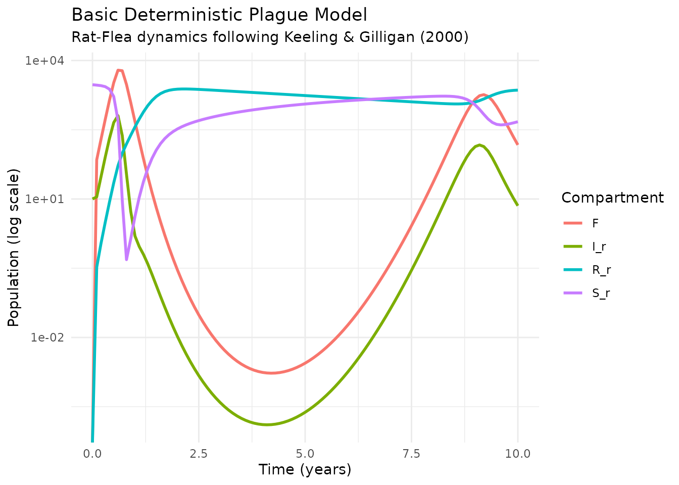

Model Analysis

Basic Reproduction Number

The basic reproduction number $R_0$ determines whether the disease can establish in the population:

# Calculate R0 using package function
R0 <- calculate_R0(params)
cat("Basic Reproduction Number (R₀):", round(R0, 3), "\n")
#> Basic Reproduction Number (R₀): 698.016

if (R0 > 1) {
  cat("✓ R₀ > 1: Disease can invade the population\n")
} else {
  cat("✗ R₀ < 1: Disease will die out\n")
}
#> ✓ R₀ > 1: Disease can invade the population

# Compare different parameter scenarios
scenarios <- c("keeling-gilligan", "modern-estimates", "historical")
R0_comparison <- data.frame(
  Scenario = scenarios,
  R0 = sapply(scenarios, function(x) calculate_R0(load_scenario(x)))
)
print(R0_comparison)
#>                          Scenario       R0
#> keeling-gilligan keeling-gilligan 581.6568
#> modern-estimates modern-estimates 684.9290
#> historical             historical 596.0916

Phase Portrait Analysis

Phase portraits reveal the system’s dynamical behavior:

# Create phase portrait (S_r vs I_r)
dat <- results_tidy |>
  select(time, compartment, value) |>
  pivot_wider(names_from = compartment, values_from = value)

ggplot(dat, aes(S_r, I_r)) +
  geom_path(alpha = 0.7) +
  geom_point(data = slice(dat, 1), color = "green", size = 3) +  # Start
  geom_point(data = slice(dat, n()), color = "red", size = 3) +   # End
  labs(
    title = "Phase Portrait: Susceptible vs Infected Rats",
    subtitle = "Green = start, Red = end",
    x = "Susceptible Rats (S_r)",
    y = "Infected Rats (I_r)"
  ) +
  theme_minimal()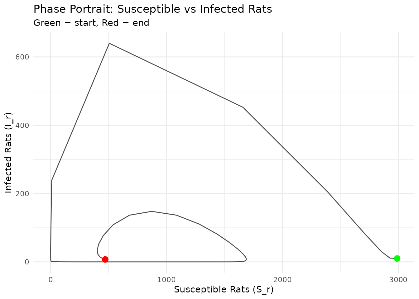

Seasonal Deterministic Model

Environmental seasonality affects plague dynamics through flea population cycles. We extend the basic model to include seasonal forcing:

seasonal_plague_model <- suppressMessages(odin::odin({
  # State variables (same as basic model)
  initial(S_r) <- K_r - I_ini
  initial(I_r) <- I_ini  
  initial(R_r) <- 0
  initial(N) <- K_f
  initial(F) <- 0

  # Total rat population
  T_r <- S_r + I_r + R_r  

  # Force of infection for humans
  lambda_h <- F * exp(-a * T_r)
  output(lambda_h) <- lambda_h  

  # Seasonal forcing on flea carrying capacity
  season_t <- interpolate(day, season, 'spline')
  K_f_seasonal <- K_f * (1 + seasonal_amplitude) ^ season_t
  output(K_f_seasonal) <- K_f_seasonal

  # Rat population dynamics (unchanged from basic model)
  deriv(S_r) <- r_r * S_r * (1 - T_r/K_r) +                
                r_r * R_r * (1 - p) -                       
                d_r * S_r -                                 
                beta_r * (S_r/T_r) * F * (1 - exp(-a*T_r))

  deriv(I_r) <- beta_r * (S_r/T_r) * F * (1 - exp(-a*T_r)) -
                (d_r + m_r) * I_r

  deriv(R_r) <- r_r * R_r * (p - T_r/K_r) +   
                m_r * g_r * I_r -              
                d_r * R_r                      

  # Flea dynamics with seasonal carrying capacity
  deriv(N) <- r_f * N * (1 - N/K_f_seasonal) +       # Seasonal logistic growth
              F * (1 - exp(-a*T_r)) / T_r            # Free fleas finding rats

  deriv(F) <- (d_r + m_r * (1 - g_r)) * I_r * N -   # Free infected fleas from dead rats
              d_f * F                                # Free flea deaths

  # Parameters from package system
  K_r <- user()      # Rat carrying capacity
  r_r <- user()      # Rat population growth rate 
  p <- user()        # Probability of inherited resistance
  d_r <- user()      # Natural death rate of rats
  beta_r <- user()   # Rat infection rate from fleas
  a <- user()        # Flea search efficiency
  m_r <- user()      # Infected rat mortality rate
  g_r <- user()      # Probability rat survives infection
  r_f <- user()      # Flea reproduction rate
  K_f <- user()      # Base flea carrying capacity per rat
  d_f <- user()      # Death rate of free fleas
  I_ini <- user()    # Initial infected rats
  
  # Seasonal forcing parameters
  seasonal_amplitude <- user()  # Amplitude of seasonal forcing
  day[] <- user()              # Vector of days for interpolation
  season[] <- user()           # Vector of seasonal values
  dim(day) <- user()
  dim(season) <- user()
}))
#> ── R CMD INSTALL ───────────────────────────────────────────────────────────────
#> * installing *source* package ‘odin38e1bca9’ ...
#> ** this is package ‘odin38e1bca9’ version ‘0.0.1’
#> ** using staged installation
#> ** libs
#> using C compiler: ‘gcc (Ubuntu 13.3.0-6ubuntu2~24.04) 13.3.0’
#> gcc -std=gnu2x -I"/opt/R/4.5.1/lib/R/include" -DNDEBUG   -I/usr/local/include    -fpic  -g -O2  -UNDEBUG -Wall -pedantic -g -O0 -fdiagnostics-color=always -c odin.c -o odin.o
#> gcc -std=gnu2x -I"/opt/R/4.5.1/lib/R/include" -DNDEBUG   -I/usr/local/include    -fpic  -g -O2  -UNDEBUG -Wall -pedantic -g -O0 -fdiagnostics-color=always -c registration.c -o registration.o
#> gcc -std=gnu2x -shared -L/opt/R/4.5.1/lib/R/lib -L/usr/local/lib -o odin38e1bca9.so odin.o registration.o -L/opt/R/4.5.1/lib/R/lib -lR
#> installing to /tmp/Rtmp15OO1Z/devtools_install_1f8078031447/00LOCK-file1f804cd2494f/00new/odin38e1bca9/libs
#> ** checking absolute paths in shared objects and dynamic libraries
#> * DONE (odin38e1bca9)

Seasonal Model Analysis

# Load parameters and add seasonal forcing
params <- load_scenario("keeling-gilligan")
params$seasonal_amplitude <- 0.3  # 30% seasonal variation

# Create seasonal forcing (sinusoidal pattern)
days <- seq(0, 365, by = 1)
seasonal_pattern <- sin(2 * pi * days / 365)

# Add seasonal data to parameters
params$day <- days
params$season <- seasonal_pattern
params$I_ini <- 10    # Initial infected rats
params$K_r <- 3000    # Rat carrying capacity

# Create seasonal model
model_seasonal <- seasonal_plague_model$new(user = params)

# Run over multiple years to see seasonal effects
times_seasonal <- seq(0, 5, by = 0.01)  # 5 years, high resolution
results_seasonal <- model_seasonal$run(times_seasonal)

# Convert to tidy format
results_seasonal_tidy <- results_seasonal |>
  tibble::as_tibble() |>
  pivot_longer(-t, names_to = "compartment", values_to = "value") |>
  rename(time = t)

# Plot showing seasonal effects
results_seasonal_tidy |>
  filter(compartment %in% c("I_r", "F", "K_f_seasonal")) |>
  ggplot(aes(time, value, color = compartment)) +
  geom_line(linewidth = 1) +
  scale_y_log10() +
  labs(
    title = "Seasonal Plague Model",
    subtitle = "Effects of seasonal flea carrying capacity variation",
    x = "Time (years)", 
    y = "Population (log scale)",
    color = "Compartment"
  ) +
  theme_minimal()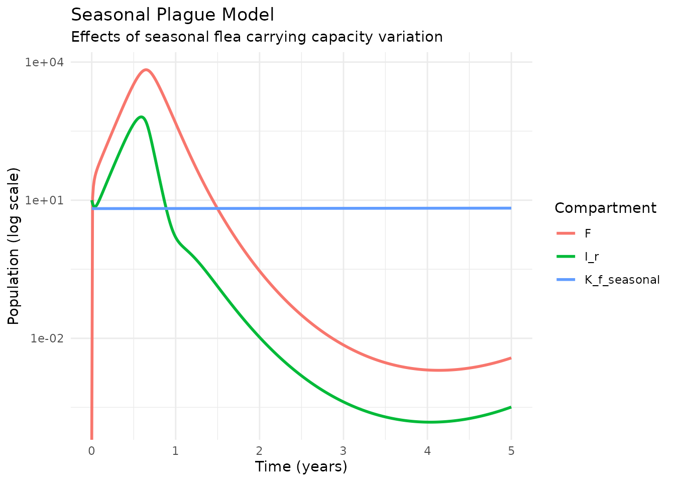

Human-Extended Model

The model can be extended to include human populations, important for understanding plague’s impact on human societies:

human_plague_model <- suppressMessages(odin::odin({
  # Rat state variables
  initial(S_r) <- K_r - I_ini
  initial(I_r) <- I_ini  
  initial(R_r) <- 0
  initial(N) <- K_f
  initial(F) <- 0
  
  # Human state variables  
  initial(S_h) <- K_h
  initial(I_h) <- 0
  initial(R_h) <- 0

  # Total populations
  T_r <- S_r + I_r + R_r
  T_h <- S_h + I_h + R_h

  # Forces of infection
  lambda_r <- beta_r * (S_r/T_r) * F * (1 - exp(-a*T_r))  # Rats
  lambda_h <- beta_h * F * exp(-a * T_r)                   # Humans
  output(lambda_h) <- lambda_h

  # Rat population dynamics (unchanged)
  deriv(S_r) <- r_r * S_r * (1 - T_r/K_r) +                
                r_r * R_r * (1 - p) -                       
                d_r * S_r - lambda_r

  deriv(I_r) <- lambda_r - (d_r + m_r) * I_r

  deriv(R_r) <- r_r * R_r * (p - T_r/K_r) +   
                m_r * g_r * I_r - d_r * R_r

  # Flea dynamics (unchanged)
  deriv(N) <- r_f * N * (1 - N/K_f) + F * (1 - exp(-a*T_r)) / T_r
  deriv(F) <- (d_r + m_r * (1 - g_r)) * I_r * N - d_f * F

  # Human population dynamics
  deriv(S_h) <- r_h * (S_h + R_h) * (1 - T_h/K_h) - d_h * S_h - lambda_h

  deriv(I_h) <- lambda_h - (d_h + m_h) * I_h

  deriv(R_h) <- m_h * g_h * I_h - d_h * R_h

  # Parameters
  K_r <- user()      # Rat carrying capacity
  r_r <- user()      # Rat population growth rate 
  p <- user()        # Probability of inherited resistance
  d_r <- user()      # Natural death rate of rats
  beta_r <- user()   # Rat infection rate from fleas
  a <- user()        # Flea search efficiency
  m_r <- user()      # Infected rat mortality rate
  g_r <- user()      # Probability rat survives infection
  r_f <- user()      # Flea reproduction rate
  K_f <- user()      # Flea carrying capacity per rat
  d_f <- user()      # Death rate of free fleas
  I_ini <- user()    # Initial infected rats
  
  # Human parameters
  K_h <- user()      # Human carrying capacity  
  r_h <- user()      # Human population growth rate
  d_h <- user()      # Natural death rate of humans
  beta_h <- user()   # Human infection rate from fleas
  m_h <- user()      # Human recovery rate
  g_h <- user()      # Probability human survives infection
}))
#> ── R CMD INSTALL ───────────────────────────────────────────────────────────────
#> * installing *source* package ‘odin5d49a224’ ...
#> ** this is package ‘odin5d49a224’ version ‘0.0.1’
#> ** using staged installation
#> ** libs
#> using C compiler: ‘gcc (Ubuntu 13.3.0-6ubuntu2~24.04) 13.3.0’
#> gcc -std=gnu2x -I"/opt/R/4.5.1/lib/R/include" -DNDEBUG   -I/usr/local/include    -fpic  -g -O2  -UNDEBUG -Wall -pedantic -g -O0 -fdiagnostics-color=always -c odin.c -o odin.o
#> odin.c: In function ‘odin_metadata’:
#> odin.c:207:18: warning: unused variable ‘internal’ [-Wunused-variable]
#>   207 |   odin_internal *internal = odin_get_internal(internal_p, 1);
#>       |                  ^~~~~~~~
#> gcc -std=gnu2x -I"/opt/R/4.5.1/lib/R/include" -DNDEBUG   -I/usr/local/include    -fpic  -g -O2  -UNDEBUG -Wall -pedantic -g -O0 -fdiagnostics-color=always -c registration.c -o registration.o
#> gcc -std=gnu2x -shared -L/opt/R/4.5.1/lib/R/lib -L/usr/local/lib -o odin5d49a224.so odin.o registration.o -L/opt/R/4.5.1/lib/R/lib -lR
#> installing to /tmp/Rtmp15OO1Z/devtools_install_1f80c7b58fb/00LOCK-file1f80487b3d12/00new/odin5d49a224/libs
#> ** checking absolute paths in shared objects and dynamic libraries
#> * DONE (odin5d49a224)

Human Model Analysis

# Load parameters including human parameters
params_human <- load_scenario("historical")  # Use historical parameters for medieval scenario
print(params_human)
#> 🦠 Plague Scenario (historical)
#> 📄  Biological parameters for historical plague outbreaks (14th-17th centuries) 
#> 📚 Source:  Historical analysis and paleoepidemiology 
#> 
#> 🐀 Rat Population Parameters:
#>   r_r    =    6.000  # Rat population growth rate (per year)
#>   d_r    =    0.150  # Natural death rate of rats (per year)
#>   p      =    0.980  # Probability of inherited resistance
#> 
#> 🦟 Flea Parameters:
#>   K_f    =    5.000  # Flea carrying capacity per rat
#>   r_f    =   15.000  # Flea reproduction rate (per year)
#>   d_f    =    8.000  # Death rate of free fleas (per year)
#>   a      =    0.003  # Flea search efficiency
#> 
#> 🔬 Disease Parameters:
#>   beta_r =    6.000  # Rat infection rate from fleas (per year)
#>   m_r    =   25.000  # Infected rat mortality rate (per year)
#>   g_r    =    0.010  # Probability rat survives infection
#> 
#> 👤 Human Parameters:
#>   r_h    =    0.030  # Human population growth rate (per year)
#>   d_h    =    0.080  # Natural death rate of humans (per year)
#>   beta_h =    0.015  # Human infection rate from fleas
#>   m_h    =   35.000  # Human recovery rate (per year)
#>   g_h    =    0.050  # Probability human survives infection
#> 
#> ⚙️  Other Parameters:
#>   mu_r   =    0.020  # Rat movement rate (per year)
#>   mu_f   =    0.005  # Flea movement rate (per year)
#>   seasonal_amplitude =    0.300  # 
#> 
#> 📈 Basic Reproduction Number (R₀):  596.092 ✅ (Disease can spread)

# Add initial conditions for human model
params_human$I_ini <- 10     # Initial infected rats
params_human$K_r <- 3000     # Rat carrying capacity
params_human$K_h <- 5000     # Human carrying capacity

# Create human model
model_human <- human_plague_model$new(user = params_human)

# Simulate Black Death scenario (5 years)
times_human <- seq(0, 5, by = 0.01)
results_human <- model_human$run(times_human)

# Convert to tidy format
results_human_tidy <- results_human |>
  tibble::as_tibble() |>
  pivot_longer(-t, names_to = "compartment", values_to = "value") |>
  rename(time = t)

# Plot human dynamics
results_human_tidy |>
  filter(compartment %in% c("S_h", "I_h", "R_h")) |>
  mutate(compartment = case_when(
    compartment == "S_h" ~ "Susceptible Humans",
    compartment == "I_h" ~ "Infected Humans", 
    compartment == "R_h" ~ "Recovered Humans"
  )) |>
  ggplot(aes(time, value, color = compartment)) +
  geom_line(linewidth = 1) +
  labs(
    title = "Human Population Dynamics in Plague Outbreak",
    subtitle = "Historical parameters representing medieval conditions",
    x = "Time (years)", 
    y = "Human Population",
    color = "Compartment"
  ) +
  theme_minimal()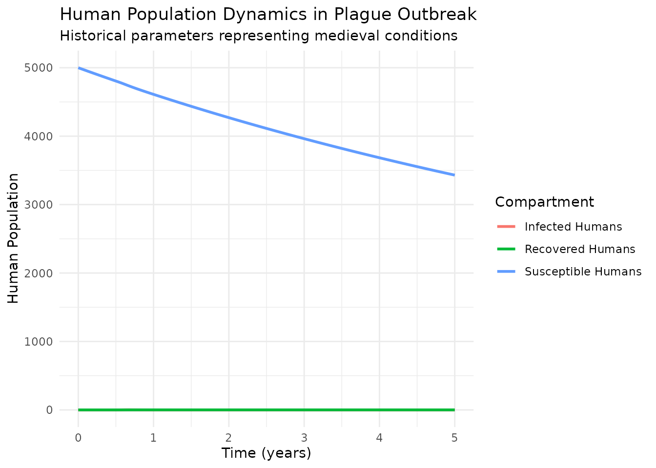


# Calculate mortality impact
final_human_pop <- results_human_tidy |>
  filter(compartment %in% c("S_h", "I_h", "R_h"), time == max(time)) |>
  summarise(final_total = sum(value)) |>
  pull(final_total)

initial_human_pop <- params_human$K_h
mortality_rate <- (initial_human_pop - final_human_pop) / initial_human_pop * 100

cat("Historical plague scenario mortality:", round(mortality_rate, 1), "%\n")
#> Historical plague scenario mortality: 31.4 %

Parameter Comparison

Understanding how different parameter sets affect model behavior:

# Compare all available parameter sets
param_sets <- c("keeling-gilligan", "modern-estimates", "historical", "defaults")
comparison_results <- list()

for (param_set in param_sets) {
  params <- load_scenario(param_set)
  params$I_ini <- 10    # Add initial conditions
  params$K_r <- 3000    # Add carrying capacity
  model <- basic_plague_model$new(user = params)
  
  results <- model$run(seq(0, 8, by = 0.1))
  results_tidy <- results |>
    tibble::as_tibble() |>
    pivot_longer(-t, names_to = "compartment", values_to = "value") |>
    rename(time = t) |>
    mutate(parameter_set = param_set)
  
  comparison_results[[param_set]] <- results_tidy
}

# Combine all results
all_results <- do.call(rbind, comparison_results)

# Plot comparison of infected rats
all_results |>
  filter(compartment == "I_r") |>
  ggplot(aes(time, value, color = parameter_set)) +
  geom_line(linewidth = 1) +
  scale_y_log10() +
  labs(
    title = "Parameter Set Comparison: Infected Rat Dynamics",
    subtitle = "Different historical and modern parameter estimates",
    x = "Time (years)", 
    y = "Infected Rats (log scale)",
    color = "Parameter Set"
  ) +
  theme_minimal()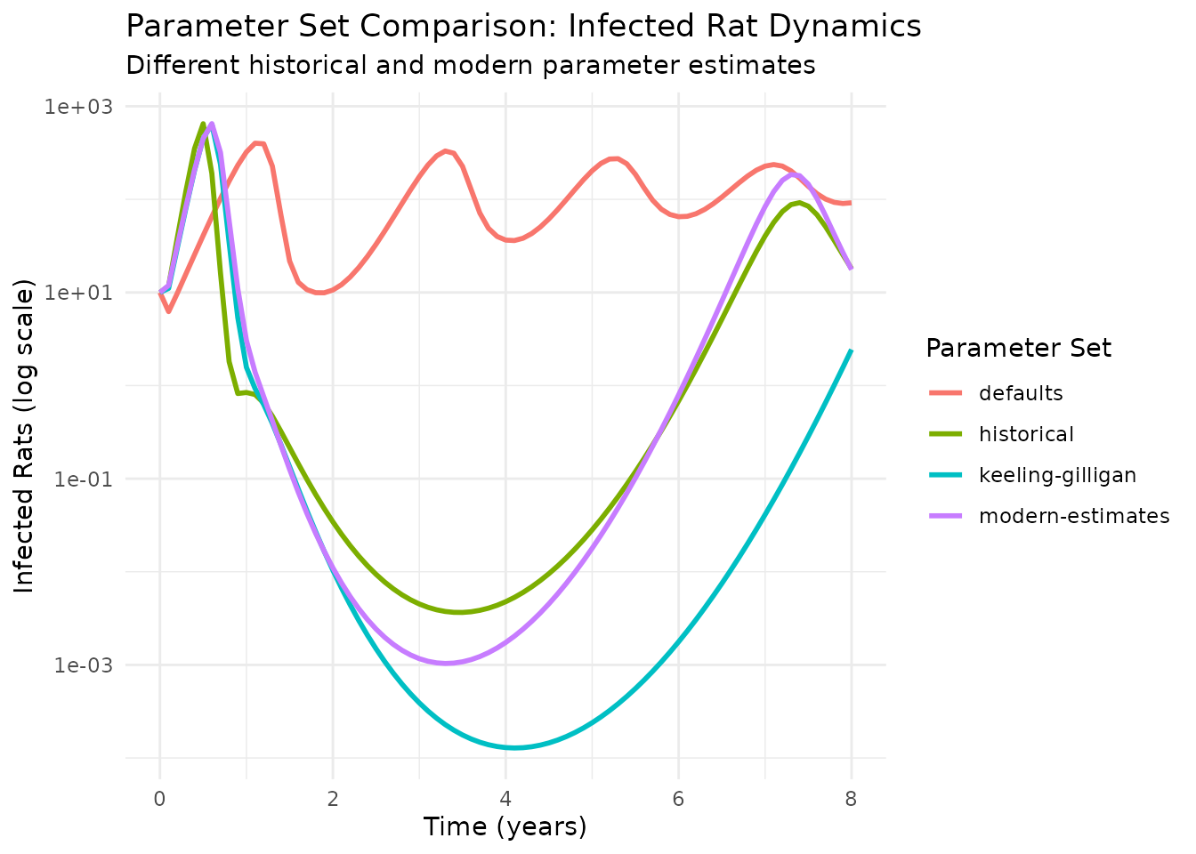


# Summary table of key characteristics
param_summary <- data.frame(
  Parameter_Set = param_sets,
  R0 = sapply(param_sets, function(x) round(calculate_R0(load_scenario(x)), 3)),
  Peak_Infected = sapply(param_sets, function(x) {
    params <- load_scenario(x)
    params$I_ini <- 10    # Add initial conditions
    params$K_r <- 3000    # Add carrying capacity
    model <- basic_plague_model$new(user = params)
    results <- model$run(seq(0, 8, by = 0.1))
    round(max(results[, "I_r"]), 0)
  })
)

print(param_summary)
#>                     Parameter_Set      R0 Peak_Infected
#> keeling-gilligan keeling-gilligan 581.657           640
#> modern-estimates modern-estimates 684.929           651
#> historical             historical 596.092           649
#> defaults                 defaults 581.657           401

Comparative Analysis

Model Behavior Across Scenarios

Different parameter sets represent different historical periods and epidemiological contexts:

Keeling-Gilligan: Original model parameters from foundational paper
Modern-estimates: Contemporary parameter values based on recent outbreaks
Historical: Medieval parameters representing Black Death conditions
Defaults: Package default values for general use

Key Insights

R₀ Variation: Different parameter sets produce varying epidemic potential
Peak Dynamics: Outbreak severity depends critically on transmission parameters
Temporal Patterns: Seasonal forcing creates cyclical outbreak patterns
Human Impact: Historical parameters suggest severe population impacts

Appendix: Interactive Model Explorer

For hands-on exploration of model behavior, the package provides an interactive gadget:

# Launch interactive plague model explorer
# This opens a Shiny gadget for parameter exploration
explore_plague_model()

The gadget allows you to:

Adjust parameters using sliders for all model parameters
Visualize results with multiple plot types (time series, phase portraits)
Compare scenarios by modifying parameters and seeing real-time updates
Export parameters for use in your own analyses

To use the gadget:

Run explore_plague_model() in your R console
Adjust parameters using the sliders in the left panel
Click “Run Simulation” to update the plots
Use different tabs to see various visualizations
Click “Done” to return modified parameters to your workspace

Note: The interactive gadget requires the shiny and miniUI packages.

Summary

This vignette has presented the mathematical foundations of deterministic plague models, implementing:

Core Models

Basic deterministic model: Fundamental rat-flea dynamics
Seasonal model: Environmental forcing through flea cycles
Human-extended model: Population impacts on human societies

Key Features

Mathematical rigor: Full differential equation formulations with biological interpretation
Package integration: Uses yersinia parameter management system
Historical context: Parameters representing different epidemiological periods
Interactive exploration: Gadget-based parameter investigation

Educational Value

These deterministic models provide: - Theoretical foundation for understanding plague transmission mechanisms - Mathematical framework for epidemiological analysis - Historical perspective on plague’s societal impact - Reference implementation for comparison with advanced stochastic models

For operational plague modeling and realistic population dynamics with stochasticity, use the main yersinia package functions described in the introductory vignette.

References

Keeling, M. J., & Gilligan, C. A. (2000). Metapopulation dynamics of bubonic plague. Nature, 407(6806), 903-906.
Stenseth, N. C., et al. (2008). Plague: past, present, and future. PLoS Medicine, 5(1), e3.
Bramanti, B., et al. (2019). Assessing the origins of the European Plagues following the Black Death. Proceedings of the National Academy of Sciences, 116(28), 13931-13940.

yersinia package

2025-09-10